Projected Density of States
Here at the FAMAlab we make use of electronic structure codes which give us huge amount of data, sometimes to handle this big amount data is very anoying, so we make use of softwares which enable us to plot with different styles. It is a routine to make this sort of plots in the lab.
- First make a DOS calculation in VASP as in the past tutorial.- Then use the texas utility to split the projected atomic density.
- This will generate n number of files which are related with the n number of atoms you have on your system. In the same order of the POSCAR file.
- This will generate n number of files which are related with the n number of atoms you have on your system. In the same order of the POSCAR file.
- To add the atoms you want in your projected DOS here at the lab we have elaborated a python script which adds all orbitals from the atoms selected.
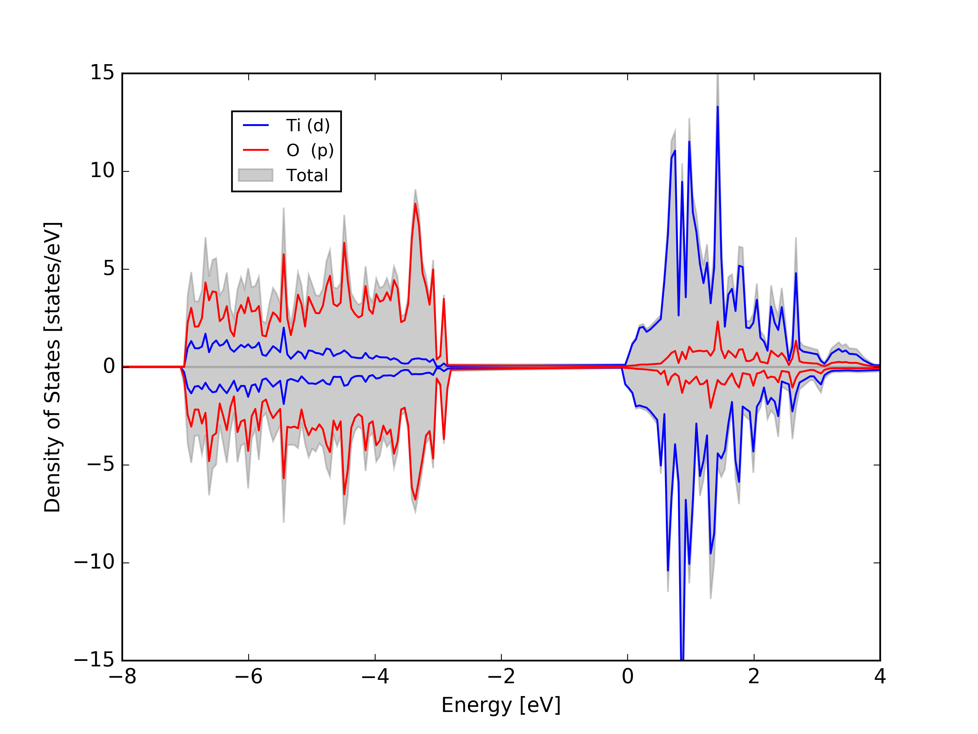
Example: TiO2 density of states
For the next examples we will use this data:[user@andromache directory]$ wget http://molphys.org/matplotlib_tutorial/plot_files/dos_plot/dosfiles.tar.gz [user@andromache directory]$ tar -zxvf dosfiles.tar.gz [user@andromache directory]$ ls DOS1 DOS2 DOS3 DOS4 DOS5 DOS6 DOS7 DOS8 DOS9 DOS10 DOS11 DOS12 [user@andromache directory]$ python sum_dos.py 1 12 > total_dos.dat [user@andromache directory]$ python sum_dos.py 1 4 > ti_dos.dat [user@andromache directory]$ python sum_dos.py 5 12 > ox_dos.dat
Now that we have the required files we create our source file to plot
import matplotlib.pyplot as pl
import numpy as np
# Load data with numpy libraries
total = np.loadtxt('total_dos.dat')
ti = np.loadtxt('ti_dos.dat')
ox = np.loadtxt('ox_dos.dat')
# Columns delimiters are simply blank spaces

#Plot Figure
#----------------------------------
fig = pl.figure(1)
ax1=pl.subplot()
           column 0   vs  column 7
ax1.fill(total[:,0], total[:,7], label=''Total up', alpha=0.6, color='gray')
ax1.fill(total[:,0], total[:,8], label=''Total down', alpha=0.6, color='gray')
ax1.plot(ti[:,0], ti[:,5], label=''Ti (d) up', lw='1.2', color='blue')
ax1.plot(ti[:,0], ti[:,6], label=''Ti (d) down', lw='1.2', color='blue')
ax1.plot(ox[:,0], ox[:,3], label=''O  (d) up', lw='2.0', color='red')
ax1.plot(ox[:,0], ox[:,4], label=''O  (d) down', lw='2.0', color='red')
# In the .dat files columns 1-2 are s up and s down orbitals
# Columns 3-4 are p up and p down, 5-6 are d, and 7-8 are the total density.