FAMAlab: DOS plots

26 April 2018

Ploting Density of States

This type of plots are very common in our area of investigation. But to plot it is not so easy, first you have to split total DOS in partial atomic density, and then to compare between different surfaces you have to make a multiplot. This require time and creativity, here we show some tips and tricks to acomplish this task. First we are going to show how to make a DOS and partial DOS, and then a multiplot of DOS's.

Generate the DOS files

The following instructions are only for VASP code. In this example we are using anatase (101).

To generate the following plots you need to download:
INCAR, POSCAR, POTCAR, KPOINTS

- After you relax the geometry of your system you have to generate the charge file to get the DOS. To generate the CHGCAR and CHG, make a single point geometry using the next instructions on the INCAR file.

#General
  System = TiO2      #Title
  PREC   = NORMAL    
  ENCUT  = 400       #Oxigen ENCUT
  ISTART = 0         #New Job
  ICHARG = 2         #Initial Charge from atoms
  LWAVE  = .FALSE.   #Wavecar is not written
  LCHARG = .TRUE.    #Final charge is written
  ISPIN  = 2         #Spin polarized
#Electronic Relaxation instructions
  NELM   = 30; NELMIN= 2; NELMDL= 10 
  EDIFF  = 1.0E-05   #Force stop criteria must be strong for DOS
  LREAL  = .TRUE.    #Real Space Projection
  IALGO  = 48        #Normal-Blocked Davidson
  VOSKOWN = 1        #1-VWN for exact correlation
#Ionic Relaxation
  EDIFFG = -1.0E-02  #stopping-criterion for IOM
  NSW    = 0         #number of steps for IOM; 0 for single point
  IBRION = -1        #ionic relax: 0-MD 1-quasi-New 2-CG -1 single point
  ISIF   = 2         #stress and relaxation 2-relax ionic 3-relax ionic and cell
  ISMEAR = 0

- In order to have more points on the DOS, you need a larger k-point mesh, in this example we are using a 6x6x1 because it is a surface.

- After you run and generate the CHG and CHGCAR, you must do a DOS calculation. Create a new folder and paste in it: CHGCAR, CHG, INCAR, POSCAR, POTCAR and KPOINTS.

- Change and add the following instructions on the INCAR file. Everything else gets the same.

#General
  ISTART = 1         #Job continuation
  ICHARG = 11         #Reads the charge from a file
#DOS related values
   ISMEAR = -5; SIGMA = 0.10  #broadening in eV -4-tet -1-fermi 0-gaus, -5=DOS
    RWIGS = 1.217  0.820      #Wigner-Seitz radio of atoms involved as apear on POSCAR
    EMIN = -30.0              #Minimum range energy for DOS carefull must have decimals
    EMAX = 15.0               #Maximum range energt for DOS carefull must have decimals
    NEDOS = 800               #Number of DOS sample sites
    LORBIT = 11               #Instruction to construct the partial DOS
    NPAR = 1                  #DOS calculation does not run in pararell

- Once you run it, VASP will generate the output files such as OUTCAR, PROCAR, DOSCAR among others. To generate the plots with gnuplot you have to split the total DOSCAR file, so please download the utilities created by the university of texas in this direction http://theory.cm.utexas.edu/vtsttools/scripts.html.

- Use the split_dos utility to separate the total DOS into atomic DOS. Be sure you are in the same directory that your vasp output files.

[user]$ split_dos

This will generate many DOS files as atoms are in the unit cell. For example if you have 32 atoms on your POSCAR, there will be 32 files labeled as DOSn. The order of the atoms is the same as in the POSCAR, if you put first 10 atoms of iron and then 20 of oxigen, DOS1 will be the projected density of the first iron, and DOS15 will be the projected density of the fifth oxigen.

Ploting Total DOS

You can skip the previus step and download the files here: dos_files.tar.gz

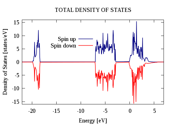
Now to plot the total density of states change the name file DOS0 to DOS0.dat which contains the total sum of states. First column is the energy, second are the spin up states, and the third are the spin down states of the system.

Use the general gnuplot template and modify the data you want to plot, in this case we are plotting all spin up and spin down states.

Also you can download this gnuplot template here: tdos_png.p. It will generate a png image.

  plot "DOS0.dat" using 1:2 title "Spin up" with lines ls 5 , \
       "DOS0.dat" using 1:3 title "Spin down" with lines ls 10;

Projected Density of State

You can divide the total DOS into the atoms states which contribute. The split_dos script divides the contribution of the total dos per atom, as said it before. For instance if we want to see the contribution of oxigen atoms into the total DOS, we sum all oxygen atoms states and plot it in the same graphic that the total DOS. To sum the atoms states download the next python script:"SORRY THIS PYTHON CODE IS UNDER REVISION, we recomend to use p4v utility".

- Check that the DOSn files has no a comment line, split dos sometimes generates the first line as a comment, delete the line comment.

- Select the atoms that you want to analize, in this case we want to see the contribution of all Ti into the Total DOS. Create a sum.inp file with the atoms, for this unit cell we have 4 Ti and 8 O. So for Ti sum.inp must look like the following.

DOS1
DOS2
DOS3
DOS4

- Sum the projected DOS per atoms with the python script

python sum_dos.py >> ti_dos.dat

- Do the same for the oxygen atoms. Modify the sum.inp file with:

DOS5
DOS6
DOS7
DOS8
DOS9
DOS10
DOS11
DOS12

- Then sum this 8 oxygen atoms.

python sum_dos.py >> o_dos.dat

- Files *.dat contains 7 columns, first is the energy zone, second and third are the s up/down states, the next 2 columns are the p up/down states, and finally the last two are the d up/down states.

- Now we can plot the projected DOS.

# Color line styles
set style line 5   lt 1  lw 1.2 pt 1 ps  0.9 lc  rgb "black"
set style line 10  lt 1  lw 0.9 pt 2 ps  1.1 lc  rgb "red"
set style line 11  lt 1  lw 0.9 pt 3 ps  1.1 lc  rgb "navy"

  plot "DOS0.dat"   using 1:2 title "Total DOS" with lines ls 5 , \
       "DOS0.dat"   using 1:3 title "" with lines ls 5, \
       "ti_dos.dat" using 1:6 title "Ti (d)" with lines ls 10, \
       "ti_dos.dat" using 1:7 title "" with lines ls 10, \
       "o_dos.dat"  using 1:4 title "O (p)" with lines ls 11, \
       "o_dos.dat"  using 1:5 title "" with lines ls 11;

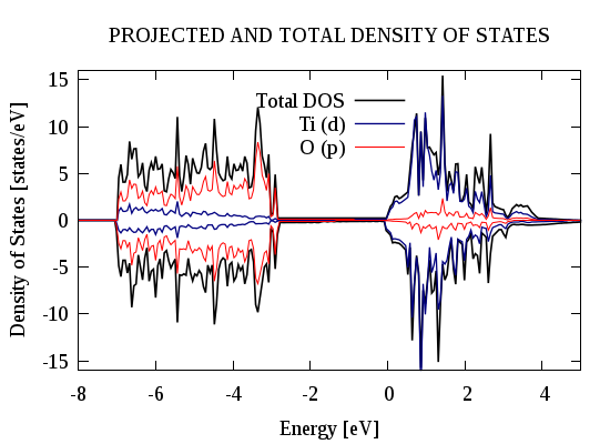
- Download this template here: proj_dos.p

Grayscale PDOS

# Grayscale PDOS
set style line 5   lt 1  lw 1.2 pt 1 ps  0.9 lc  rgb "gray80"
set style line 10  lt 1  lw 1.0 pt 2 ps  1.1 lc  rgb "gray50"
set style line 11  lt 5  lw 1.4 pt 3 ps  1.1 lc  rgb "gray20"

  plot "DOS0.dat"   using 1:2 title "Total DOS" with filledcurve y1=0 ls 5 , \
       "DOS0.dat"   using 1:3 title "" with filledcurve y1=0 ls 5, \
       "ti_dos.dat" using 1:6 title "Ti (d)" with lines ls 10, \
       "ti_dos.dat" using 1:7 title "" with lines ls 10, \
       "o_dos.dat"  using 1:4 title "O (p)" with lines ls 11, \
       "o_dos.dat"  using 1:5 title "" with lines ls 11;

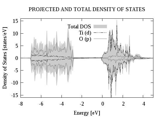
- Download this template here: gray_pdos.p